
In this article, we will implement linear regression from scratch with NumPy, then will implement it with PyTorch and then we will use torch’s built-in functions. In the first two, we will do all of the implementations ourselves to understand how it works step by step, and finally, we will use PyTorch's built-in function so we will not deal with calculating derivatives, etc …
I highly recommend you to read my previous article Understanding Gradient before jumping into this article assumes you have knowledge of how gradient descent works.
As we have discussed in the previous article, gradient descent is an optimization function and it does it by using the derivative of the function. When we implement linear regression, our goal is to minimize the error; which means that we need to find the derivate of the error function.
A common function used in linear regression to calculate error is: mean squared error.
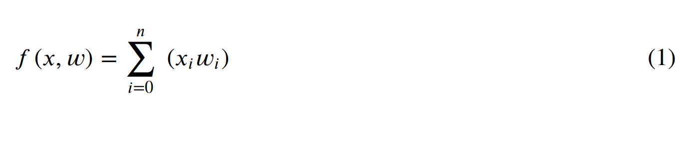
Before moving forward, let’s define the linear regression function.
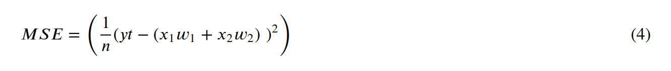
Now, we can define the mean squared error

, where yt shows the true results and yp shows the predicted results
Calculating Derivatives
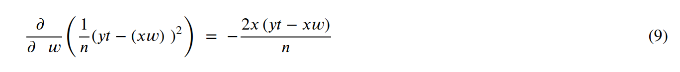
The error function we want to minimize is MSE which has been shown with equation (2).
For the sake of simplicity, let’s say we have only two input columns; then our f function becomes:

So, MSE becomes the following equation when we replace yp with the f function:
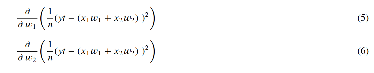
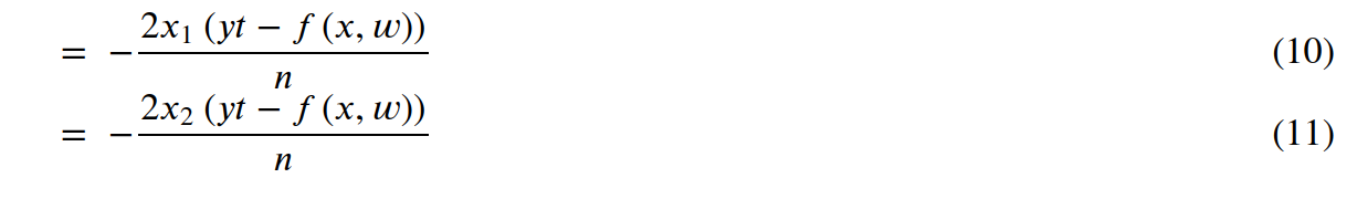
What we need to do is to calculate the partial derivatives for w₁ and w₂:
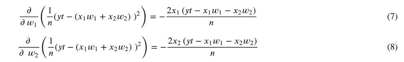
And, the derivatives become:
And, finally, we can generalize those:
To be honest, as long as you understand why we need derivatives, I believe it is not a problem not to know how to solve all those equations. You can use a tool like https://www.symbolab.com/solver/partial-derivative-calculator.
When we look at equations (7) and (8), we see that −𝑥₁𝑤₁−𝑥₂𝑤₂ which is basically -f(x,w). So, we can rewrite those equations:
And, finally, equation (9) can be written as:

Implementation with NumPy
In this section, we will implement linear regression with gradient descent and we will use the equations that we just went through.
- X is the input and y_true is the output that we will use to train machine learning.
- w_true is the one we used to calculate y_true and, those are the values that the ML algorithm does not know and tries to learn with gradient descent.
- f function is the implementation of the equation (1)
- mse function is the implementation of the equation (2)
import numpy as np
w_true = np.array([
[10],
[20]
])
X = np.array([
[1, 2],
[3, 4],
[5, 6]
])
def f(X, w):
return np.sum(np.dot(X, w), 1)
y_true = f(X, w_true)
def mse(y_true, y_pred):
np.mean((y_true-y_pred)**2)
y_true
array([ 50, 110, 170])
The following code block uses equations (10) and (11). df_w0 and df_w1 is used to store the values of the results of the equations (10) and (11), respectively. The problem with the following code block is; it can't scale for more than 2 weights. If the input variables have more than 2 columns, it will not work.
w variable is the variable that we are trying to predict. First, we initialize it and we update it with each iteration and use it again in the next iteration.
learning_rate = 0.0001
nepochs=1000000
w = np.array([
[0.1],
[0.1]
])
for _ in range(nepochs):
df_w0 = (-2*np.dot(X[:,0],(y_true-f(X, w))))/len(X)
df_w1 = (-2*np.dot(X[:,1],(y_true-f(X, w))))/len(X)
w[0] = w[0] - (learning_rate*df_w0)
w[1] = w[1] - (learning_rate*df_w1)
w
array([[10.00000008],
[19.99999994]])
The following code block is the generalized version of the previous code block that can be used with the input variables that have more than 2 columns, and it uses the equation (12).
learning_rate = 0.0001
nepochs=1000000
w = np.array([
[0.1],
[0.1]
])
for _ in range(nepochs):
df = (-2*np.dot(X.T,(y_true-f(X, w))))/len(X)
w -= learning_rate*df.reshape(w.shape)
w
array([[10.00000008],
[19.99999994]])
Implementation with PyTorch tensors
The previous sections show how linear regression is implemented with NumPy. Now, it is time to implement it with PyTorch tensor. But, we will continue implementing functions ourselves instead of using PyTorch's built-in error function, etc…
The following code is very similar to what you have seen in the previous section but with torch tensors. For example; you can use see that we are importing torch import torch as T and then converting NumPy arrays to tensors with those two lines:
X = T.from_numpy(X)
w = T.from_numpy(w)
import numpy as np
import torch as T
w_true = np.array([
[10.],
[20.]
])
X = np.array([
[1., 2.],
[3., 4.],
[5., 6.]
])
X = T.from_numpy(X).float()
w_true = T.from_numpy(w_true).float()
def f(X, w):
return T.matmul(X, w)
def mse(y_true, y_pred):
return T.sum((y_true-y_pred)**2)/len(y_true)
y_true = f(X, w_true)
In the next code block, where training happens, you will see that we are initializing w values with w = T.tensor([0.,0.], requires_grad=True). requires_grad tells that we will calculate gradient for w variable and as we covered so far, w variable is the variable that we are trying to figure out.
The line mse(y_true, y_pred).backward() tells that calculate the error and then calculate the gradient. The following 3 lines are used to calculate the new w variable, which will be used in the next iteration. By default, PyTorch does a cumulative calculation so we need to clean the gradient with the line w.grad.zero_() :
with T.no_grad():
w -= w.grad*learning_rate
w.grad.zero_()
learning_rate = 0.0001
nepochs=1000000
w = T.tensor([
[0.],
[0.]
], requires_grad=True)
for _ in range(nepochs):
y_pred = f(X, w)
mse(y_true, y_pred).backward()
with T.no_grad():
w -= w.grad*learning_rate
w.grad.zero_()
w
tensor([[10.0429],
[19.9661]], requires_grad=True)
Implementation with PyTorch built-in functions
Wewill start playing a different game in this section. We will start using PyTorch's built-in MSELoss function, SGD function, and Linear function. Here is what we will do;
- we will replace f with T.nn.Linear
- we will replace mse with T.nn.MSELoss
- we will replace w -= w.grad*learning_rate with optimizer.step() where optimizer is T.optim.SGD.
We will no more calculate the gradient ourselves and calculate the new w ourselves. Also, instead of using f variable, we will name it model which is a common keyword because we are trying to find the parameters of a model and those parameters are basically w values.
We will not initialize w anymore because when we define the model with T.nn.Linear, model parameters (w values) are assigned randomly at the beginning and in each iteration, they are assigned new variables with optimizer.step().
We will not clean the gradient ourselves as we did previously with w.grad.zero_(), we will ask the optimizer to clean it with optimizer.zero_grad() function.
And, finally, we will not print out w because we did not define w, we will just print out the model.parameters() which contains w.
learning_rate = 0.0001
nepochs=1000000
mse = T.nn.MSELoss()
model = T.nn.Linear(2, 1, bias=False)
optimizer = T.optim.SGD(model.parameters(), lr=learning_rate)
for _ in range(nepochs):
y_pred = model(X.float())
mse(y_pred.float(), y_true.reshape(-1, 1).float()).backward()
optimizer.step()
optimizer.zero_grad()
list(model.parameters())
[Parameter containing:
tensor([[10.0429, 19.9661]], requires_grad=True)]
Conclusion
In this article, we explained how linear regression works and implemented it in 3 different ways:
- First, we explained how linear regression works and calculated the derivatives, but to understand it we referenced the previous article about gradient descent titled Understanding Gradient.
- Then, we implemented linear regression in 3 different ways:
- We implemented with NumPy and we implemented all necessary functions (derivatives, gradient descent, loss function, f function) ourselves
- After that, we implemented it with PyTorch tensors and the only difference was using tensor instead of NumPy arrays.
- Finally, we implemented it using PyTorch's functions so we did not need to implement the functions ourselves, we just used them.

.jpg)

