
Gradient Descent algorithm is the hero behind the family of deep learning algorithms. When an ml algorithm in this family runs, it tries to minimize the error between the training input and predicted output. This minimization is done by optimization algorithms and gradient descent is the most popular one. Let’s move with examples.
Let’s say you have these input & output pairs:
input:
[
[1,2],
[3,4]
]
output:
[
[50],
[110]
]
We can quickly estimate that; if we multiply the input values by [10, 20], we can have the output as shown above.
1*10 + 2*20 = 50
3*10 + 4*20 = 110
When a machine learning algorithm starts running, it assigns random values and makes a prediction. Let’s say it assigned [1,2] values:
1*1 + 2*2 = 5
3*1 + 4*2 = 11
Once it has predictions, it calculates the error: the difference between the real data and the predicted data. There are many ways to calculate the error and they are called loss functions. Since this is not the topic of this article, we will skip this part. For now, let’s call this value as e.
Once we have this value; the optimization algorithm starts showing itself and it sets new values which replace the initial random values. And, the loop continues until a condition is met. The condition can be;
- loop n times
- loop until e is smaller than a value
Roughly, the algorithm is;
- #1 initialize random weights
- #2 make prediction with weights
- #3 calculate the difference via loss function
- #4 calculate the new weights via optimization formula/function
- #5 go to step #2
As I have mentioned in the previous paragraph; the most popular optimization algorithm is the gradient descent algorithm and I will try to explain the mechanics behind it in this article.
Intuition behind Gradient Descent
It could be hard to understand gradient descent without understanding gradient. So, let’s focus on what gradient is. The gradient shows the direction of the greatest change of a scalar function. The gradient calculation is done with derivatives, so let’s start with a simple example. To calculate the gradient, we just need to remember some linear algebra calculations from high school because we need to calculate derivatives. We will go with a simple example.
Let’s say we want to find the minimum point of f(x)=x^2. The derivative of that function is df(x)=2*x. The gradient of f(x) at point.
- x=-10 is df(-10)=-20.
- x=1 is df(1)=2
Now let’s visualize f(x) and those x=-10 and x=1 points.
import torch
import numpy as np
import seaborn
def f(x):
return x**2
def df(x):
return 2*x
def visualize(f, x=None):
xArray = np.linspace(-10, 10, 100)
yArray = f(xArray)
seaborn.lineplot(x=xArray, y=yArray)
if x is not None:
assert type(x) in [np.ndarray, list] # x should be numpy array or list
if type(x) is list: # if it is a list, convert to numpy array
x = np.array(x)
y = f(x)
seaborn.scatterplot(x=x, y=y, color='red')
visualize(f, x=[-10, 1])
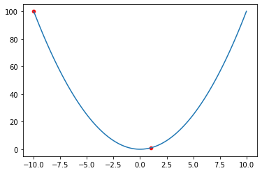
Think about this: the red dot at x=-10 does not know the surface it stands on and it only knows the coordinates of where it stands and that the gradient of itself which is -20. And the other red dot at x=1 does not know the surface it stands on and it only knows the coordinates of where it stands and that the gradient of itself which is 2.
By having only this information: we can say that the red dot at x=-10 should make a bigger jump than x=1 because it has a bigger absolute gradient value. The sign shows the direction. - shows that the red dot at x=-10 should move to the right and the other one should move to the left.
In summary; the red dot at x=-10 (gradient: -20) should make a bigger jump and the red dot at x=1 (gradient: 2) should make a smaller jump to the left. Let's list what we know so far:
- We know that the jump length should be proportional to the gradient, but what is that value exactly? We don’t know. So, let’s just say that red points should move with the length of alpha*gradient where alpha is just a parameter.
- We also know that if the gradient is negative it should move to the right (to the positive direction on the x-axis) and if the gradient is positive it should move to the left (to negative direction on the x-axis). We can say that sign of the gradient shows the opposite direction of what the red dot wants to move.
When combining all this knowledge, we can say that the new location of the red dot should be calculated with the following formula:
x = x - gradient * alpha
Gradient Descent with numpy
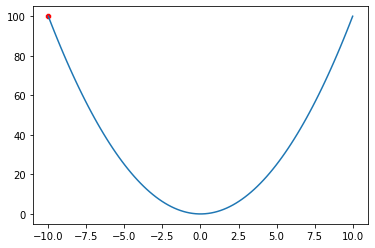
In this section, I will implement what I have explained in the previous section, with numpy. Let’s start with visualizing f(x)=x^2 function and x=-10 point.
visualize(f, x=[-10])
The following code block just implements the whole logic that I have explained. I added comments to the code to explain the details.
def gradient_descent(x, nsteps=1):
#collectXs is an array to store how x changed in each iteration,
#so we can visualize it later
collectXs = [x]
#learning_rate is the value that we mentioned as alpha in previous section
learning_rate = 1e-01
for _ in range(nsteps):
#that following one line is the does the real magic
#the next value of x is calculated by subtracting the gradient*learning_rate by itself
#the intuation behind this line is in the previous section
x -= df(x) * learning_rate
collectXs.append(x)
#we return a tuple that contains
#x -> recent x after nsteps
#collectXs -> all the x values that was calculated so far
return x, collectXs
Before running gradient descent with 1000 steps, let’s just run it twice, one step at a time to see how x evolves. we start with x=-10 and it evolves to x=-8. We know that when x=0 that is the minimum point, so, yes it is evolving in the correct direction.
x=-10
x, collectedXs = gradient_descent(x, nsteps=1)
print(x)
-8.0
The next step will start at x=-8. After running gradient for 1 step, we can see it goes to x=-6.4. So far so good.
x, collectedXs = gradient_descent(x, nsteps=1)
print(x)
-6.4
Let’s run it 1000 times.
x, collectedXs = gradient_descent(x, nsteps=1000)
print(x)
-7.873484301831169e-97
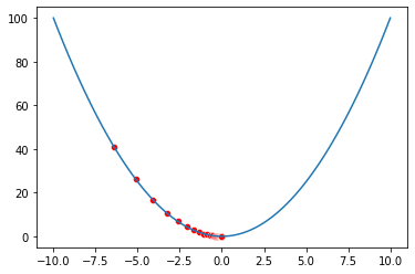
The final result is almost 0. Let’s visualize all steps and see how the red dot changes with each step.
visualize(f, x=collectedXs)
Gradient Descent with pytorch tensor
The following function is the gradient descent implementation with pytorch tensors. I provided the explanation of the code with the code comments.
def gradient_descent(x, nsteps=1):
#x is a tensor and to save a copy of the data in the list,
#we have to use .detach().numpy() function of the tensor
#https://pytorch.org/docs/stable/generated/torch.Tensor.detach.html
collectXs = [x.detach().numpy()]
learning_rate = torch.tensor(1e-01)
for _ in range(nsteps):
#now, something is changing with numpy implementation
#f(x) is the same f(x) that we used in numpy implementation but it uses x as tensor
#when we use f(x).backward(), it calculates gradient; so that we can access x.grad
#we do not need to calculate the gradient with df(x) anymore
f(x).backward()
with torch.no_grad():
#this is the same logic as shown in the previous section
#this time, we are using x.grad which was calculate via f(x).backward()
x -= x.grad*1e-01
#we have to clean the gradient in x tensor with .zero_() function
#if we don't, tensor just accumulates the results
x.grad.zero_()
collectXs.append(x.detach().numpy().copy())
return x, collectXs
When we define a pytorch tensor, we can define if its gradient will be calculated or not; this is defined with requires_grad=True/False variable. The goal of this article is to show how gradient works, so we will go with requires_grad=True parameters.
As I have done in the previous section, I run gradient descent twice to see if we have the same results.
x = torch.tensor(-10., requires_grad=True)
x, _ = gradient_descent(x)
x
tensor(-8., requires_grad=True)
tensor(-6.4000, requires_grad=True)
We just verified that it has the same results: -8 and -6.4. Let's run it 1000 times and visualize how x changed in each iteration.
x, collectedXs = gradient_descent(x, nsteps=1000)
visualize(f, x=collectedXs)

Gradient Descent with pytorch sgd function
In this section, we will implement gradient descent once again but this time we will use pytorch’s sgd function. We will not calculate the derivative function df(x) and we will not do the calculation for x=x-grad*alpha to calculate the next x.
def gradient_descent(x, nsteps=1):
optim = torch.optim.SGD([x], lr=1e-01)#, momentum=0, weight_decay=0, nesterov=False)
collectXs = [x.detach().numpy()]
for _ in range(nsteps):
#calculate gradient
f(x).backward()
#x-=x*grad*learning_rate
optim.step()
#clean grads
optim.zero_grad()
collectXs.append(x.detach().numpy().copy())
return x, collectXs
As usual, we will run twice; 1 step each time, and then check the results.
x = torch.tensor(-10., requires_grad=True)
x, _ = gradient_descent(x)
x
tensor(-8., requires_grad=True)
x, _ = gradient_descent(x)
x
tensor(-6.4000, requires_grad=True)
We just verified the results and everything seems fine. It is time to visualize how x changed in each step.
x, collectedXs = gradient_descent(x, nsteps=1000)
visualize(f, x=collectedXs)
Conclusion
In this article; I tried to explain what gradient descent is, how gradient descent works and implemented it in 3 different ways.
- Gradient descent is the hero behind deep learning algorithms and the most popular optimization algorithm. Optimization algorithms are used to minimize the error between the actual output and the predicted output.
- We tried to see how the red dot navigates in an environment it does not know about. It only knows the coordinates of where it is and its gradient. We showed that the red dot can find the minimum point by using only this knowledge and gradient descent algorithm.
- We did 3 implementations:
- ▹ with numpy (we used gradient descent formula and derivative of function)
- ▹ with pytorch tensor (we used gradient descent formula but did not calculate derivative ourselves)
- ▹ with pytorch sgd function (we did not use used gradient descent formula and did not calculate derivative ourselves)

.jpg)

