
This article is the 3rd part of the Understanding Series. The first two articles are:
Logistic regression differs from linear regression. Linear regression is used when the target value is a continuous value and logistic regression is used when the target value is a categorical value. Linear regression algorithm is a regression algorithm and logistic regression is a classification algorithm.
In this article, we will implement logistic regression with PyTorch:
- First, we will implement binary logistic regression; binary logistic regression is used when the output label is binary (0 or 1). We will go into details of binary cross-entropy and sigmoid functions which are used as loss and activation functions for binary logistic regression
- Then, we will implement multi-class logistic regression; which is used when the output label can have more than 2 outputs. We will go into details of cross-entropy and softmax functions which are used as loss and activation functions for binary logistic regression
It is highly recommended that you read the first two articles of the series before moving on.
Binary Logistic Regression
We have seen that linear regression is formulated as:
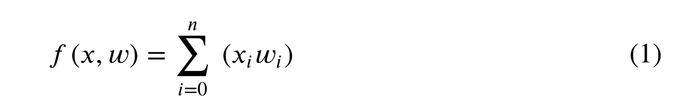
Logistic regression has a small difference that makes a big impact and it is shown as:
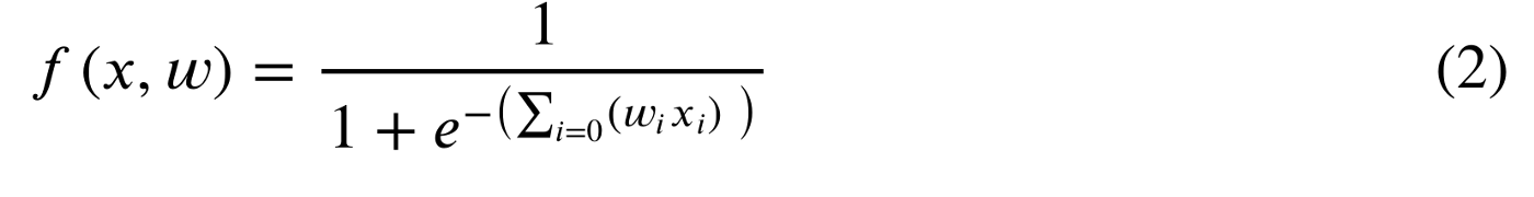
The equation shown with 1/(1+e⁻ˣ) is called a sigmoid function. And as it can be seen in equation (2), it is used to wrap the output of equation (1). The responsibility of the sigmoid function is to convert the result of the equation (1) to a value between 0 and 1. Let’s demonstrate it with some python code.
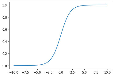
In the above code, we generated x values between -10 and 10 and then calculated y values with the sigmoid function. As you have seen, it just converts the values between 0 and 1. 0 and 1 will be used as the output of the binary logistic regression and the output is interpreted as the probability.
As we have known from previous articles, we will use gradient descent to optimize loss function; but, here is the question: what is the loss function for binary logistic regression if we are using sigmoid function? MSE (mean squared error) was the loss function that was used to calculate the difference between predicted values and real target values when it was linear regression.
For binary logistic regression; we will use BCE (Binary Cross Entropy).
Understanding BCE
BCE equation is shown in equation (3).
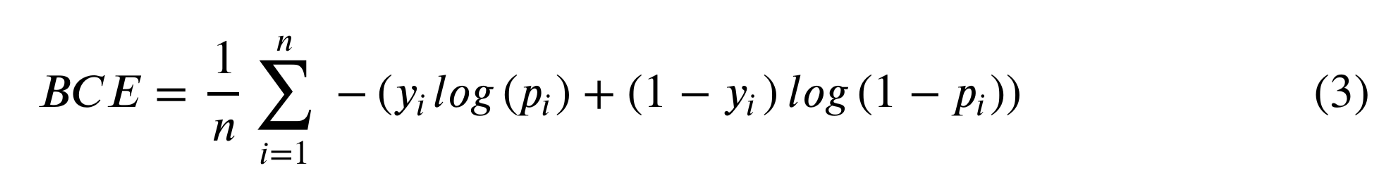
The left part of the formula (yᵢlog(pᵢ)) is triggered when yᵢ=1 and the right part of the formula ((1−yᵢ)log(1−pᵢ)) is triggered when yᵢ=0. Just to understand it; let’s focus on the left part of the equation which is only triggered when yᵢ=1. The formula becomes:
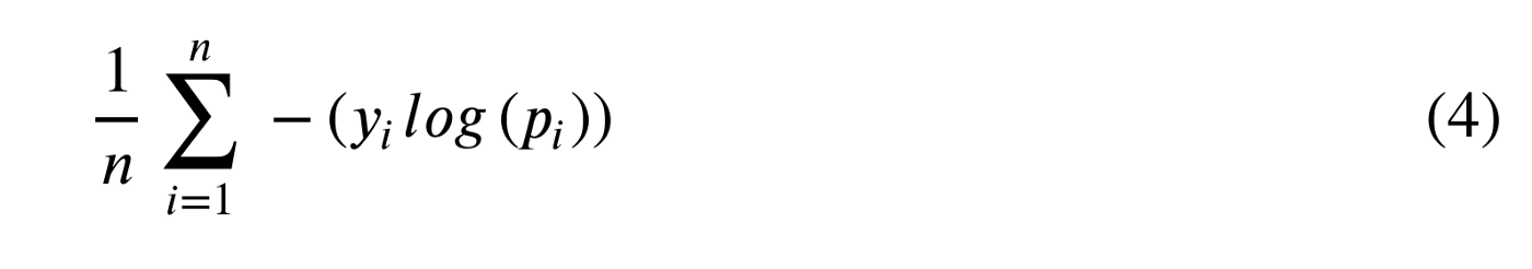
Since yᵢ is always 1, we can see that BCE becomes the average of -log(pᵢ). Let’s try to understand why we are using -log(pᵢ) by visualizing it.
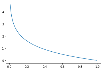
As we have seen with the MSE function for linear regression, an error function should give us smaller errors if the predicted values and the real values are converging. That is what we are having with -log(pᵢ). If the real value is 1 and the prediction has a value that is closer to 1, -log(pᵢ) is returning a smaller value.
Now, let’s also visualize -log(1-pᵢ)
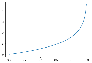
-log(1-pᵢ) is the mirror view of -log(pᵢ). While -log(pᵢ) is returning smaller values while the real value is 1, -log(1-pᵢ) is returning smaller values if the real value is 0.
When we combine those two formulas, we end up with the formula defined in equation (3).
For more information on BCE, you can read:
- Understanding binary cross-entropy / log loss: a visual explanation
- Binary Cross Entropy/Log Loss for Binary Classification
Let’s continue with the implementation details.
Implementation
Instead of downloading a dataset, we will use sklearn’s make_classification function to create a classification dataset. We will create a dataset of 10000 rows with 20 features and 2 classes for binary classification.
We will also use train_test_split function to split the data. We will use 90% of the data for training and 10% of the data for validation. The validation dataset will be used in each iteration to see the accuracy of the model; how model performance evolves with each iteration on unseen data.
You can see that we are using sigmoid function in forward function. So, forward function is doing the calculation shown with equation (2).
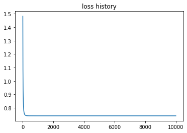
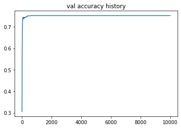
The following code block is used for the training. We are defining the loss function and the optimizer. As an addition to the values that we will use for training; we also created two variables loss_history and val_accuracy_history. Those variables will store the values for loss and accuracy on the validation dataset so we can visualize it later.
The training steps are no more different than what we have shown in previous articles:
- make a prediction (y_pred = model(X_train.float()))
- calculate the loss (loss = loss_f(y_pred.float(), y_train.reshape(-1, 1).float()))
- calculate gradient (loss.backward())
- run optimizer function to assign new model parameters (optimizer.step())
- and, continue iterating.
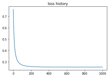
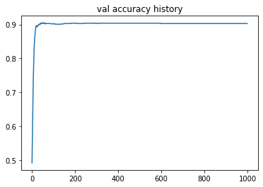
It’s time to see how the model evolved during the training by visualizing the loss_history and val_accuracy_history variables.
In the following charts, we can see that loss is going down and accuracy on validation is going up.
We have seen how binary logistic regression works, it is time to jump into multi-class logistic regression
Multi-Class Logistic Regression
Multi-Class logistic regression is used when the target value has more than 2 values.
As usual, the algorithm steps for multi-class logistic regression are no more different than the linear regression and binary logistic regression. In each iteration;
- it makes prediction
- calculates gradient
- calculates the new model parameters
Now, let’s focus on the differences.
Output Dimension
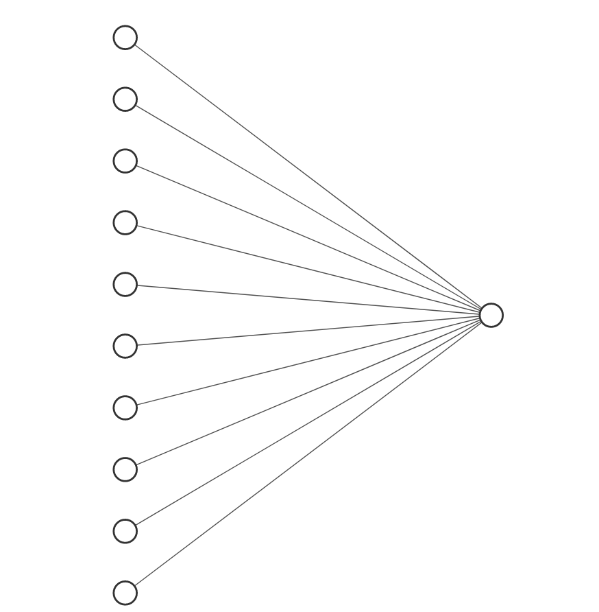
For binary classification and linear regression, we always had 1 output which means the output dimension was 1. The following is an example of a neural network with 10 input variables and 1 output variable.
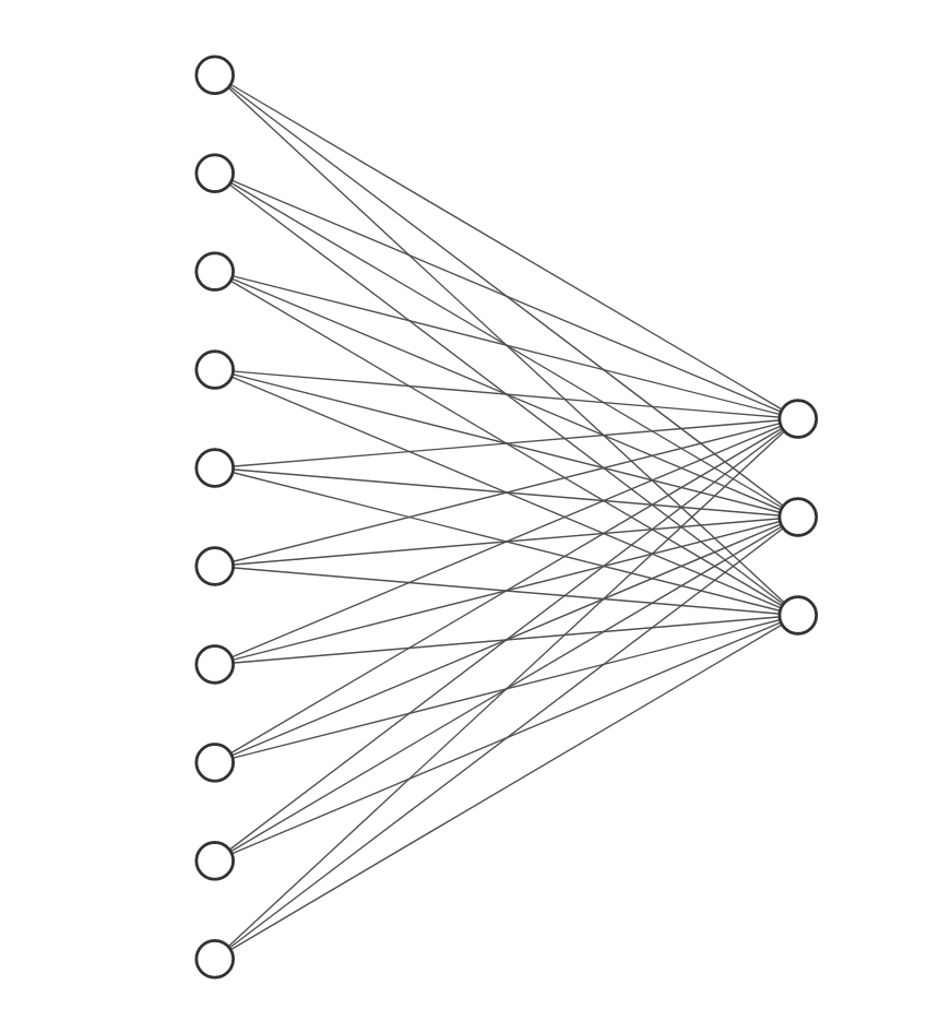
For multi-class logistic regression, the output dimension will be the number of classes. The following is an example of a neural network with 10 input variables and 3 output variables.
We will use sklearn’s OneHotEncoder function to convert the target classes to n-array representation.
Activation Function
For binary logistic regression, we used sigmoid function. For multi-class logistic regression, we will use softmax activation function. But, here is the difference;
- we used the sigmoid function in forward function because the loss function (BCE) required the output of thesigmoidfunction.
- we will NOT use softmax function in forward function because the loss function (Cross-Entropy Loss) we will use (PyTorch's Cross-Entropy Loss implementation) requires the linear output. The PyTorch implementation of the Cross-Entropy Loss first calculates softmax itself.
Loss Function
For binary logistic regression, we used BCE (Binary Cross Entropy). For multi-class logistic regression, we will use Cross Entry (CE) function. CE is the generalized version of BCE. We have shown BCE with equation (3). The CE function is shown with the following equation:
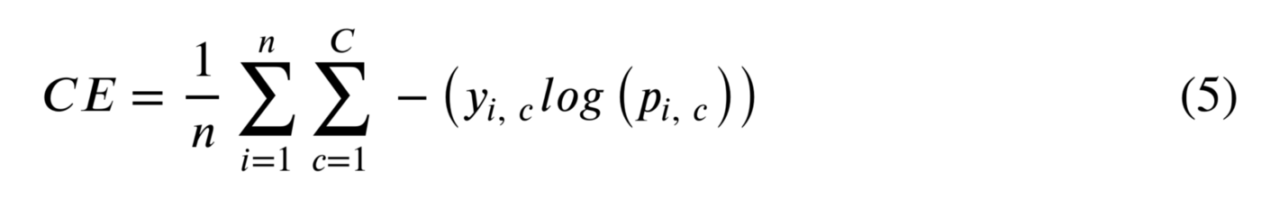
where C is the number of classes.
CE is just the generalized version of BCE. In BCE, we did not use ∑, because we had only 2 classes and we added the values by using +. With CE, we are looping for each class prediction and calculating the sum for each row. After that, we are calculating the average of cross-entropy values of all rows with 1⁄n ∑.
As we have mentioned, cross-entropy requires the output of softmax. Let’s say our linear function returns a value of y_pred=[.01, 0.1, 0.2] for a 3-class problem. And, let's assume the real class of the row is the 3rd one which is shown as [0, 0, 1].
Softmax converts y_pred to probabilities and probabilities for each class is [0.29252603 0.35373698 0.35373698]. cross_entropy function calculates the entropy for 1 single row (as you have noticed y_pred is just 1 row). And the result of this function is 1.039.
The 2nd next block uses PyTorch's CrossEntropyLoss function. We can see that it also has the same result: 1.039. So, we can verify that our cross_entropy function which was implemented with NumPy is correct.
Implementation
We understood how Cross-Entropy works and we understood how SoftMax works; the next step is moving with PyTorch implementation.
Conclusion
Inthis article, we implemented binary logistic regression and multi-class logistic regression with PyTorch. Not only that, but we also explained how they work.
- Binary logistic regression uses sigmoid as activation function and binary cross-entropy as loss function. We demonstrated the intuition behind those functions by visualizing them.
- Multi-class logistic regression uses softmax as the activation function and the cross-entropy as loss function. We explained how cross-entropy is the generalized version is binary cross-entropy, implemented with NumPy, and compared the result with PyTorch's cross-entropy implementation. Also, we explained how multi-class logistic regression’s neural network architecture differs from binary logistic regression and visualized it.

.jpg)

