Understanding Image Classification: Convolutional Neural Networks

In this article, we will continue from where we left: image classification. This time we will implement image classification by using a convolutional neural network (CNN) and as usual, we will implement with Pytorch. We need to learn 2 new building blocks — that we did not introduce in the previous articles — to be able to build a convolutional neural network: convolution and max pooling.

We will start the article by introducing convolution which is the most important building block on CNN and we will try to understand the intuition behind this concept. We will continue max pooling, which is a layer used after the convolution layer.

Once we have those important building blocks, we will continue introducing the CIFAR-10 dataset. This dataset has only 10 classes, which is enough to show how CNN works. Finally, we will implement CNN with PyTorch and build functions for training and evaluating the results. In the implementation phase, as a difference from the previous articles; we will use GPU and make small changes in the codebase to be able to use GPU.

Convolution

Convolution is the process of applying a function to a given input. From our image classification viewpoint, it is just applying a filter to an image. When we represent the image as a matrix; we start sliding a smaller matrix on the main matrix and do element-wise multiplication with the filter matrix and add them up. The result is a new matrix which is the image with a filter applied to it. The following animation shows this process.

In this section;

we will implement the filtering process explained above with PyTorch's Conv2d class to show how that works and explain the role of the convolution layer in a neural network
we will implement two filtering functions (one written with tensors, the other with PyTorch's Conv2d class):
a) apply_filter_with_tensor function which takes an input image and applies the filter and returns the filtered image and uses tensors
b) apply_filter_with_conv2d function which takes an input image and applies the filter and returns the filtered image and uses PyTorch's Conv2d class

During those examples; we will a filter called emboss filter.

‍

import os

import torch

import torchvision

import tarfile

from torchvision.datasets.utils import download_url

from torch.utils.data import random_split

import matplotlib.pyplot as plt

import torchvision.transforms as transforms

import seaborn

from torch import nn

from PIL import Image

import torchvision.transforms as transforms

import torch

import numpy as np

import torch.nn.functional as F

from tqdm import tqdm

‍

How Conv2d works and role of convolution in a neural network

As we have explained previously, applying a filter is only element-wise matrix multiplication and adding up all. In the following code, you can see that we are using matrix m and filter emboss.

The line print(torch.sum(emboss*m)) prints out exactly this calculation and the final result is 29. After that line of code; you can see that we are using PyTorch's Conv2d class which we will use later in neural network architecture code. The final line of the next code blocks prints out the same results.

‍

emboss = torch.tensor([

[-2, -1, 0],

[-1, 1, 1],

[0, 1, 2]

]).float()

m = torch.tensor([

[1,2,3],

[4,5,6],

[7,8,9]

]).float()

print(torch.sum(emboss*m))

c2d = nn.Conv2d(in_channels=1, out_channels=1, kernel_size=(3,3), bias=False)

c2d._parameters['weight'] = emboss.reshape(1, 1, emboss.shape[0], emboss.shape[1])

print(c2d(m.reshape(1, 1, m.shape[0],m.shape[1])))

‍

tensor(29.)
tensor([[[[29.]]]])

In the example above; we set the weights ourselves to show what Conv2d does. But, while the neural network is being trained, we are asking Conv2d to learn its weights itself that serves the final objective. In summary; we are asking neural network architecture to find the best filters that help us to achieve our image classification problem.

You can see that we are using the parameters called in_channels and out_channels. The channel keyword is borrowed from the image processing. For example; if an image is grayscaled image, it is a 1-channel image; if it is an RGB colored image, it is a 3-channel image. From a tensor perspective; we can say that it is the depth of the matrix. out_channels is the depth we want to create. As an example; we can convert a 3-channel to 10-channel image and after that point, it becomes the new feature set that will be fed to the next layer.

Image Filtering

In this section, we will implement two functions to show how image filtering works. The first implementation will use native tensor functions, the second implementation will use Conv2d class.

We will start with using the PIL library to read the image, and converting it to a tensor with transforms.ToTensor. We can see that the channel size is 1 since it is a grayscaled image.

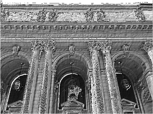
After running two functions, we can visually inspect that two functions perform identically.

‍

img = Image.open("image.jpg")

img

‍

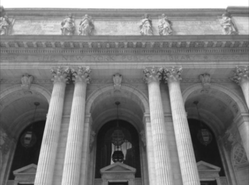
im = transforms.ToTensor()(img)

print(im.shape)

‍

torch.Size([1, 370, 498])

def apply_filter_with_tensor(im, fm):

"""

im: image matrix

fm: filter matrix

"""

new_image = torch.ones(im.shape)

for channel in range(im.shape[0]):

for i in range(im.shape[1])[1:-1]:

for j in range(im.shape[2])[1:-1]:

window = im[channel][i-1:i+2, j-1:j+2] # get the sliding window

output = torch.sum(window*fm) # multiply it by the filter

new_image[channel][i][j] = output

return new_image

new_image = apply_filter_with_tensor(im=im, fm=emboss)

transforms.ToPILImage()(new_image)

‍

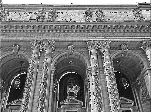
def apply_filter_with_tensor(im, fm):

"""

im: image matrix

fm: filter matrix

"""

new_image = torch.ones(im.shape)

for channel in range(im.shape[0]):

for i in range(im.shape[1])[1:-1]:

for j in range(im.shape[2])[1:-1]:

window = im[channel][i-1:i+2, j-1:j+2] # get the sliding window

output = torch.sum(window*fm) # multiply it by the filter

new_image[channel][i][j] = output

return new_image

new_image = apply_filter_with_tensor(im=im, fm=emboss)

transforms.ToPILImage()(new_image)

‍

Max Pooling

Max pooling layer is usually used after the convolution layer. It works by sliding a matrix on the main matrix and selecting the maximum value on that sliding window. It is easy to understand what max-pooling does but, why do we use max-pooling?

Experiments have shown that this process helps to increase the performance of neural networks for image classification. Andrew NG’s explains:

But I have to admit, I think the main reason people use max pooling is because it’s been found in a lot of experiments to work well, and the intuition I just described, despite it being often cited, I don’t know of anyone fully knows if that is the real underlying reason. I don’t have anyone knows if that’s the real underlying reason that max pooling works well in ConvNets. [2]

In some cases instead of max pooling, the average pooling is used which is the average of the sliding window. It all depends on the dataset, problem, performance, and the experiments.

The following code blocks show how max-pooling works by using the MaxPool2d class. We are using a 2x2 matrix on a 3x3 matrix and sliding it; and, with each iteration, we are fetching the maximum value.

m = torch.tensor([[

[1,2,3,4],

[5,6,7,8],

[9,10,11,12]

]]).float()

p = nn.MaxPool2d(2, stride=1)

p(m)

m = torch.tensor([[

[1,2,3,4],

[5,6,7,8],

[9,10,11,12]

]]).float()

p = nn.MaxPool2d(2, stride=1)

p(m)

m = torch.tensor([[

[1,2,3,4],

‍

tensor([[[ 6., 7., 8.],
[10., 11., 12.]]])

I am sure you noted the stride parameter. This shows how sliding moves. In the previous code block, it moves 1 by 1. It means; it first uses [[1,2],[5,6]] and then moves to the next one which is [[2,3],[6,7]]. If we use stride=2, it would use [[3,4],[7,8]]. The following code blocks execute max pooling with stride=2 parameter.

p = nn.MaxPool2d(2, stride=2)

p(m)

‍

tensor([[[6., 8.]]])

So far, we explained the building blocks for image classification. It is time to move on with the image classification implementation. In the next 2 sections;

we will introduce the CIFAR 10 dataset,
and, we will implement an image classification code.

CIFAR 10 dataset

CIFAR 10 dataset is a widely used dataset for machine learning research. It contains 60,000 images with a size of 32x32, in 10 classes.

Let’s start with loading the data.

train_ds = torchvision.datasets.CIFAR10(root='./data', train=True, download=True)

test_ds = torchvision.datasets.CIFAR10(root='./data', train=False, download=True)

train_ds, test_ds, train_ds[0]

‍

Files already downloaded and verified
Files already downloaded and verified

(Dataset CIFAR10
Number of datapoints: 50000
Root location: ./data
Split: Train,
Dataset CIFAR10
Number of datapoints: 10000
Root location: ./data
Split: Test,
(<PIL.Image.Image image mode=RGB size=32x32 at 0x7FDDD9FA0D90>, 6))

Ok, we have our data. As you can see, the data is in PIL format. We need to transform them into tensors so we can use them in the next steps.

The next 2 lines download train & test datasets and transform them into tensors. And, finally, we show the first image in the training dataset.

You will see that we use img.permute function. plt.imshow requires the channel to be 3rd dimension, but PyTorch tensor converts and uses the channel as the 1st dimension. That is the reason we are changing the order of the dimensions before showing it.

train_ds = torchvision.datasets.CIFAR10(root='./data', download=True, train=True, transform=transforms.ToTensor())

test_ds = torchvision.datasets.CIFAR10(root='./data', train=False, transform=transforms.ToTensor())

classes = ('airplane', 'automobile', 'bird', 'cat', 'deer', 'dog', 'frog', 'horse', 'ship', 'truck')

img, label = train_ds[0]

print('img tensor shape:', img.shape)

print('label of the shape:', classes[label])

plt.imshow(img.permute(1, 2, 0))

‍

Files already downloaded and verified
img tensor shape: torch.Size([3, 32, 32])
label of the shape: frog

<matplotlib.image.AxesImage at 0x7fddd86cff50>

In the next two code blocks;

we will implement get_loaders function which splits the training data into two parts (training and validation) and returns loader objects for training, validation, and testing datasets. We will use the training dataset’s loader object to load the dataset in batches during the training phase.
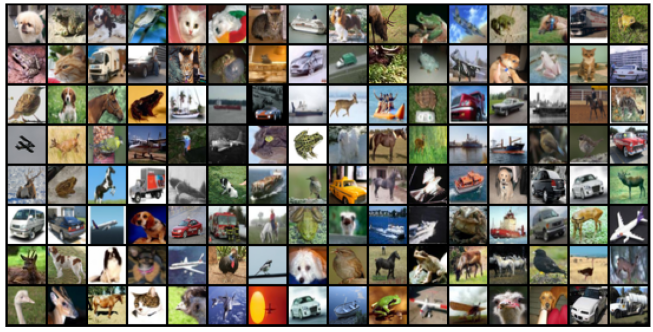
we will implement show_batch function which takes the loader as input and show the first batch of the images.

from torch.utils.data import random_split

from torch.utils.data import DataLoader

def get_loaders(train_dataset, batch_size):

n_train_ds = int(len(train_dataset)*.9)

n_val_ds = len(train_dataset) - n_train_ds

train_ds, val_ds = random_split(train_dataset, [n_train_ds, n_val_ds])

train_loader = DataLoader(train_ds, batch_size, shuffle=True)

val_loader = DataLoader(val_ds, batch_size)

test_loader = DataLoader(test_ds, batch_size)

return train_loader, val_loader, test_loader

train_loader, val_loader, test_loader = get_loaders(train_ds, 128)

‍

from torchvision.utils import make_grid

def show_batch(loader):

for images, labels in loader:

fig, ax = plt.subplots(figsize=(24, 12))

ax.set_xticks([]); ax.set_yticks([])

ax.imshow(make_grid(images, nrow=16).permute(1, 2, 0))

break

show_batch(train_loader)

‍

Training

In this section, we will start implementing the image classification with convolutional layers. Before going into implementation details, let’s see how the neural network layers look like:

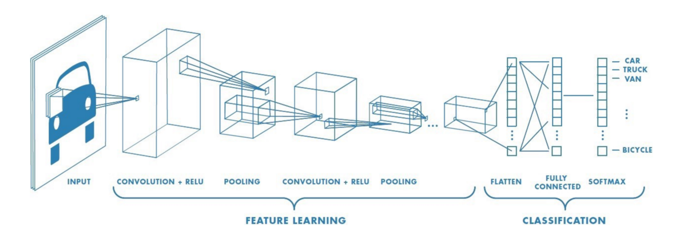
As we can see in the previous figure, we will use

convolution layers followed by ReLu activation functions
and, then, we will use max-pooling
once we have the final feature sets, we will flatten the array and connect it usual regular neural network layers.

If you have followed the previous articles, we already know how to create a model with PyTorch. In the following code block; we will create the model that we just described and as a difference from our previous articles, we will use GPU if exists.

get_device returns cuda:0 if GPU exists and is usable, if not cpu. The model will use GPU with this simple line: model.to(device).

def get_device():

if torch.cuda.is_available():

device = torch.device('cuda:0')

else:

device = torch.device('cpu') # don't have GPU

return device

device = get_device()

print(device)

class Cifar10CnnModel(nn.Module):

def __init__(self):

super().__init__()

self.network = nn.Sequential(

nn.Conv2d(3, 32, kernel_size=3, padding=1),

nn.ReLU(),

nn.Conv2d(32, 64, kernel_size=3, stride=1, padding=1),

nn.ReLU(),

nn.MaxPool2d(2, 2), # output: 64 x 16 x 16

nn.Conv2d(64, 128, kernel_size=3, stride=1, padding=1),

nn.ReLU(),

nn.Conv2d(128, 128, kernel_size=3, stride=1, padding=1),

nn.ReLU(),

nn.MaxPool2d(2, 2), # output: 128 x 8 x 8

nn.Conv2d(128, 256, kernel_size=3, stride=1, padding=1),

nn.ReLU(),

nn.Conv2d(256, 256, kernel_size=3, stride=1, padding=1),

nn.ReLU(),

nn.MaxPool2d(2, 2), # output: 256 x 4 x 4

nn.Flatten(),

nn.Linear(256*4*4, 1024),

nn.ReLU(),

nn.Linear(1024, 512),

nn.ReLU(),

nn.Linear(512, 10)

)

def forward(self, xb):

return self.network(xb)

def predict_proba(self, x):

return torch.softmax(self(x), 1)

def predict(self, x):

probs = self.predict_proba(x)

return probs.argmax(dim=1)

model = Cifar10CnnModel()

model.to(device)

‍

cuda:0

Cifar10CnnModel(
(network): Sequential(
(0): Conv2d(3, 32, kernel_size=(3, 3), stride=(1, 1), padding=(1, 1))
(1): ReLU()
(2): Conv2d(32, 64, kernel_size=(3, 3), stride=(1, 1), padding=(1, 1))
(3): ReLU()
(4): MaxPool2d(kernel_size=2, stride=2, padding=0, dilation=1, ceil_mode=False)
(5): Conv2d(64, 128, kernel_size=(3, 3), stride=(1, 1), padding=(1, 1))
(6): ReLU()
(7): Conv2d(128, 128, kernel_size=(3, 3), stride=(1, 1), padding=(1, 1))
(8): ReLU()
(9): MaxPool2d(kernel_size=2, stride=2, padding=0, dilation=1, ceil_mode=False)
(10): Conv2d(128, 256, kernel_size=(3, 3), stride=(1, 1), padding=(1, 1))
(11): ReLU()
(12): Conv2d(256, 256, kernel_size=(3, 3), stride=(1, 1), padding=(1, 1))
(13): ReLU()
(14): MaxPool2d(kernel_size=2, stride=2, padding=0, dilation=1, ceil_mode=False)
(15): Flatten(start_dim=1, end_dim=-1)
(16): Linear(in_features=4096, out_features=1024, bias=True)
(17): ReLU()
(18): Linear(in_features=1024, out_features=512, bias=True)
(19): ReLU()
(20): Linear(in_features=512, out_features=10, bias=True)
)
)

The following code block has 4 functions, including fit function which is used for training.

t2n function is used to convert tensor to NumPy array,
accuracy function is used to calculate accuracy ;)
evaluate function is used to calculate the score based on given inputs; we will use it a) to calculate the loss of validation data during training and b) to calculate the accuracy of the test dataset
fit function is used for training.

We had used SGD optimizer in our previous articles, but, experiments show that Adam optimizer provides better performance for that problem. So, we will use Adam optimizer, you are free to change and experiment and see the performance of the model when SGD is used.

def t2np(t):

if t.get_device()>=0:

return t.cpu().detach().numpy()

else:

return t.detach().numpy()

def accuracy(y_true, y_pred):

corrects = (y_true == y_pred)

return corrects.sum()/corrects.shape[0]

def evaluate(loader, eval_f, y_true_f):

ret_list = []

for batch in loader:

X, y = batch

ret = eval_f(y_true_f(X.to(device)), y.to(device))

ret_list.append(t2np(ret))

return np.mean(ret_list)

def fit(model, epochs, train_loader, val_loader, loss_func, optimizer, val_metrics):

loss_history = {'train': [], 'val': []}

val_metrics_history = {k:[] for k in val_metrics}

for epoch in tqdm(range(epochs)):

loss_history_for_batch = []

val_metrics_for_batch = {k:[] for k in val_metrics}

for batch in train_loader:

X, y = batch

loss = loss_func(model(X.to(device)), y.to(device))

loss.backward()

loss_history_for_batch.append(t2np(loss))

optimizer.step()

optimizer.zero_grad()

loss_history['train'].append(np.mean(loss_history_for_batch))

with torch.no_grad():

loss = evaluate(loader=val_loader, eval_f=loss_func, y_true_f=model)

loss_history['val'].append(loss)

for metric in val_metrics:

score = evaluate(loader=val_loader, eval_f=val_metrics[metric], y_true_f=model.predict)

val_metrics_history[metric].append(score)

return loss_history, val_metrics_history

loss_func = F.cross_entropy

optimizer = torch.optim.Adam(model.parameters(), 0.001)

val_metrics = {'accuracy': accuracy}

loss_history, val_metrics_history = fit(

model=model, epochs=10, train_loader=train_loader, val_loader=val_loader,

loss_func=loss_func, optimizer=optimizer,

val_metrics=val_metrics

)

‍

100%|██████████| 10/10 [01:57<00:00, 11.80s/it]

Here is the final part of all implementation we had so far. We will

plot the loss history on the training data during the training phase,
plot the loss history on the validation data during the training phase,
plot the accuracy of the validation data during the training phase,
and print out the accuracy on the test dataset.

def plot(loss_history):

from matplotlib import pyplot as plt

for k in loss_history:

plt.figure()

seaborn.lineplot(

x=range(len(loss_history[k])), y=loss_history[k]

).set_title(k)

plot(loss_history)

plot(val_metrics_history)

print('accuracy on test dataset:', evaluate(loader=test_loader, eval_f=accuracy, y_true_f=model.predict))

‍

accuracy on test dataset: 0.75988925

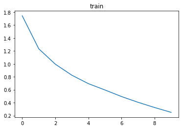
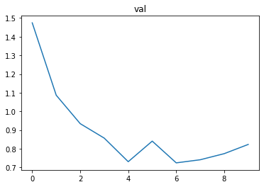
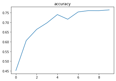
As we expect;

the loss on the training dataset and validation dataset is decreasing,
the accuracy on the validation dataset is increasing.

In just 10 iterations, we have a 75% accuracy on the test dataset — this is the dataset that we never used until this point.

Conclusion

In this article, we showed how image classification works with convolutional layers. In the 1st section, we explained what convolution is, what the role of convolution is in a neural network, and the relation of it with image filtering. We also provided python code examples to show it. In the 2nd section, we explained what max pooling is and showed how it works with a python code example. In the 3rd section, we showed CIFAR-10 dataset; how to load and transform it. And finally, in the 4th section, we trained the model — we used loaders and GPU -. In the implementation details, we implemented some helper functions to evaluate the results, convert the tensor to NumPy array and plot the results. In the end, we saw that we had 75% accuracy on the test dataset.