
In this article, we will jump into image classification. We will use the MNIST dataset which is a widely used image dataset that contains gray images of digits from 0 to 9. Image classification, as the name implies, is a classification problem and we will use logistic regression. Logistic regression has been discussed in the previous article.
First, we will start the article with understanding the MNIST dataset; we will use PyTorch's util functions to download it and matplotlib to visualize it. In previous articles, we did not train in batches; but we will do in this article and we will use PyTorch's some helper functions to help us to ease this process.
We will continue the article with the training process. We will create 3 separate models and show how they differ from each other in terms of performance; we will learn how performance changes when the model changes.
MNIST Dataset
import torch
import torchvision
from torchvision.datasets import MNIST
import matplotlib.pyplot as plt
import torchvision.transforms as transforms
import seaborn
We will start with downloading the MNIST dataset. In the following code block, the first 2 lines are used to download the training and testing dataset by using the torchvision.datasets.MNIST function. The 3rd line prints out some info about those.
As you can see the training dataset has 60K rows and the testing dataset has 10K datasets.
train_dataset = MNIST(root='data/', download=True, train=True)
test_dataset = MNIST(root='data/', train=False)
train_dataset, test_dataset
(Dataset MNIST
Number of datapoints: 60000
Root location: data/
Split: Train,
Dataset MNIST
Number of datapoints: 10000
Root location: data/
Split: Test)
Let’s print out the 1st data point to understand what it is. train_dataset[0] is a tuple where the 1st element contains the image in PIL format (python image library) and the 2nd element is the corresponding label of the image. In this example; the label is 5.
train_dataset[0]
(<PIL.Image.Image image mode=L size=28x28 at 0x7FD42A15F7D0>, 5)
Let’s visualize it and verify it.
img, label = train_dataset[0]
plt.imshow(img, cmap='gray')
print('Label:', label)
Label: 5

The data is in PIL format but we need tensor to work with for training. Thanks to PyTorch's helper functions, the transform parameter will help us. The following 2 lines download the dataset (if they do not exist locally) and transform the image to tensor.
train_dataset = MNIST(root='data/', download=True, train=True, transform=transforms.ToTensor())
test_dataset = MNIST(root='data/', train=False, transform=transforms.ToTensor())
When we unpack the first tuple of the training dataset and print out the first element, we can verify that it is a PyTorch tensor with 1x28x28 dimension. So, what does 1x28x28 mean? The first dimension shows the number of channels. 1 simply shows this is a grayscaled image. If it was an RGB image, it would be 3. The second and third dimensions show the width and height information. The dimension of the single image is 28x28.
img, label = train_dataset[0]
img.shape
torch.Size([1, 28, 28])
Training a multi-class logistic regression
In previous articles, we learned how to implement logistic regression. In this section, we will use logistic regression as we have used before but we will have some differences.
In each epoch, we used whole training dataset to calculate the gradients but in this section, we will do it by batches. For that, we will use PyTorch's DataLoader class as our helper class to load data in batches.
The following code block:
- splits the data: 90% as training data and 10% of the data as validation data (validation data will be used to calculate the accuracy of validation data for each epoch)
- creates train_loader and val_loader variables with a batch size of 128.
from torch.utils.data import random_split
from torch.utils.data import DataLoader
n_train_ds = int(len(train_dataset)*.9)
n_val_ds = len(train_dataset) - n_train_ds
train_ds, val_ds = random_split(train_dataset, [n_train_ds, n_val_ds])
batch_size = 128
train_loader = DataLoader(train_ds, batch_size, shuffle=True)
val_loader = DataLoader(val_ds, batch_size)
The following code block contains the function that is used for training. The main logic of the code block is no more different than what we have done so far in previous articles. As addition:
- we have loss_history variable which is used to store the loss value of the training dataset for each epoch
- we have val_history variable which is used to store the accuracy of the model for the validation dataset in each epoch
- and, we are doing the training in batches.
def fit(epochs, learning_rate, model, train_loader, val_loader, loss_func, val_func, opt_func=torch.optim.SGD):
optimizer = opt_func(model.parameters(), learning_rate)
loss_history = []
val_history = []
for epoch in range(epochs):
loss_history_for_batch = []
for batch in train_loader:
X, y = batch
loss = loss_func(model(X), y)
loss.backward()
loss_history_for_batch.append(loss.detach().numpy())
optimizer.step()
optimizer.zero_grad()
loss_history.append(np.mean(loss_history_for_batch))
val_history_for_batch = []
for batch in val_loader:
X, y = batch
score = val_func(y, model.predict(X))
val_history_for_batch.append(score)
val_history.append(np.mean(val_history_for_batch))
return loss_history, val_history
In the following code block, we will create a new PyTorch module. As an addition to previous implementations we did, we will also implement predict_proba and predict functions. predict_proba calculates the probability of each class by using softmax function and predict function returns the class with the biggest probability.
As we have seen in the previous section; the dimension of the images is 28x28. It means that the input dimension of the data to the logistic regression is 28x28=784. When the data comes as a 28x28 matrix, we will reshape the matrix into an array with this line: x.reshape(-1, input_size).
import torch.nn.functional as F
import numpy as np
import torch.nn as nn
input_size = 28*28
num_classes = 10
class MnistModel(nn.Module):
def __init__(self):
super().__init__()
self.linear = nn.Linear(input_size, num_classes)
def forward(self, x):
x = x.reshape(-1, input_size)
return self.linear(x)
def predict_proba(self, x):
return torch.softmax(self(x), 1)
def predict(self, x):
probs = self.predict_proba(x)
return probs.argmax(dim=1)
model = MnistModel()
model
MnistModel(
(linear): Linear(in_features=784, out_features=10, bias=True)
)
And, finally, we will define the accuracy function and run the fit function. The accuracy function will be used to calculate the accuracy of the validation dataset; it returns a number between 0 and 1 which we will interpret as x% accuracy. We will call the fit function with all the parameters we defined so far:
- epochs: we will run only 10 epochs
- learning rate: will be 0.1
- model is the model we defined with MnistModel class
- train_loader and val_loader will be used to load the data in batches
- the loss function is the cross-entropy which is used when we used multi-class logistic regression
- val_func is the accuracy function we just defined
def accuracy(y_true, y_pred):
corrects = (y_true == y_pred)
return corrects.sum()/corrects.shape[0]
loss_history, val_history = fit(
epochs=10, learning_rate=0.1, model=model,
train_loader=train_loader, val_loader=val_loader,
loss_func=F.cross_entropy, val_func=accuracy
)
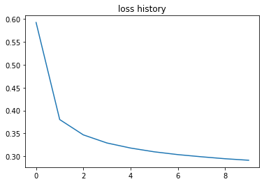
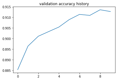
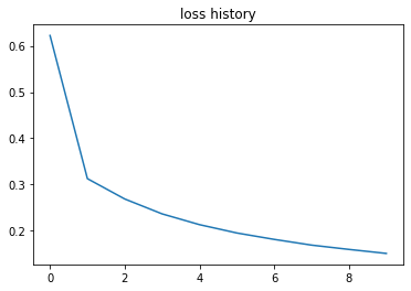
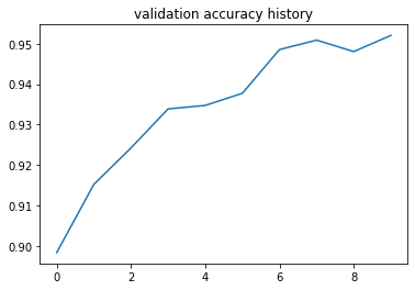
After running the training, it is time to visualize how loss and accuracy changed. The following code block is used the plot the charts and the next two charts are loss history and validation accuracy history. As expected, the loss is decreasing and accuracy is increasing. In just 10 epochs, we have more than 90% accuracy on the validation dataset.
import matplotlib.pyplot as plt
def plot(loss_history, val_history):
plt.figure()
seaborn.lineplot(x=range(len(loss_history)), y=loss_history).set_title("loss history")
plt.figure()
seaborn.lineplot(x=range(len(val_history)), y=val_history).set_title("validation accuracy history")
plot(loss_history, val_history)
Let’s see how a prediction can be done with the code we implemented. The following code block runs the forward function for the first element of the validation dataset. Once we run it, we can see that the shape of the result is 1x10. We have 10 classes, that is why we have 10 results, but we need to be careful here; the output is not the probabilities of each class yet.
x, y = val_ds[0]
model(x).shape
torch.Size([1, 10])
The following prints out the probabilities of each class. Also, it prints out the predicted class which is 1. The last line visualizes the image. And, yes, we can verify that it really is 1.
probs = model.predict_proba(x)
predicted_class = model.predict(x)
print("probs:", probs)
print("predicted_class:", predicted_class)
plt.imshow(x[0,:,:], cmap='gray')
probs: tensor([[2.7587e-06, 9.9706e-01, 1.9900e-03, 8.0092e-05, 9.8932e-05, 2.4678e-04,
4.5156e-05, 2.7545e-04, 1.9585e-04, 2.5272e-06]],
grad_fn=<SoftmaxBackward0>)
predicted_class: tensor([1])

Training a multi-class logistic regression with a hidden layer
In this section, we will continue using logistic regression and we will try to improve the performance of the model by adding a new layer. The hidden layer will have 32 nodes. This is something you can change and experiment with.
import torch.nn.functional as F
import numpy as np
class MnistModel(nn.Module):
def __init__(self):
super().__init__()
self.layer1 = nn.Linear(input_size, 32)
self.layer2 = nn.Linear(32, num_classes)
self.num_classes = num_classes
def forward(self, x):
x = x.reshape(-1, input_size)
l1 = self.layer1(x)
return self.layer2(l1)
def predict_proba(self, x):
return torch.softmax(self(x), 1)
def predict(self, x):
probs = self.predict_proba(x)
return probs.argmax(dim=1)
model = MnistModel()
model
MnistModel(
(layer1): Linear(in_features=784, out_features=32, bias=True)
(layer2): Linear(in_features=32, out_features=10, bias=True)
)
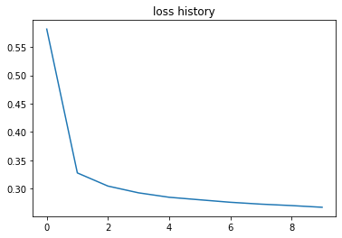
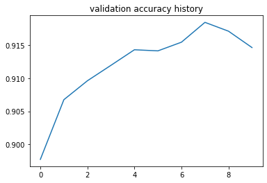
After running this neural network for 10 epochs, we can see that it has slightly better performance. But it does not mean that is it. You can continue experimenting with hyper-parameters and see how it changes.
loss_history, val_history = fit(
epochs=10, learning_rate=0.1, model=model,
train_loader=train_loader, val_loader=val_loader,
loss_func=F.cross_entropy, val_func=accuracy
)
plot(loss_history, val_history)
Training a multi-class logistic regression with hidden layer and Relu function
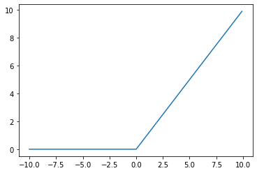
So far, we increased the accuracy value up to 92%. Can we do more? We will start using the ReLu function. ReLu function is used to convert negative numbers to zero and that is all about it. That approach seems to work well in many classification problems.
Let’s visualize the ReLu function to see how it works.
x = torch.arange(-10, 10, 0.1)
y = F.relu(x)
seaborn.lineplot(x=x, y=y)
The following code block has the same model as we have implemented in the previous section but with the ReLu function. For more information about ReLu: Finally, an intuitive explanation of why ReLU works
import torch.nn.functional as F
import numpy as np
class MnistModel(nn.Module):
def __init__(self):
super().__init__()
self.layer1 = nn.Linear(input_size, 32)
self.layer2 = nn.Linear(32, num_classes)
self.num_classes = num_classes
def forward(self, x):
x = x.reshape(-1, input_size)
l1 = F.relu(self.layer1(x))
return self.layer2(l1)
def predict_proba(self, x):
return torch.softmax(self(x), 1)
def predict(self, x):
probs = self.predict_proba(x)
return probs.argmax(dim=1)
model = MnistModel()
loss_history, val_history = fit(
epochs=10, learning_rate=0.1, model=model,
train_loader=train_loader, val_loader=val_loader,
loss_func=F.cross_entropy, val_func=accuracy
)
plot(loss_history, val_history)
And, voila, by just adding ReLu; we increased the accuracy up to 95%.
Conclusion
In this article, we explained the basics of image classification and used MNIST dataset as an example dataset to demonstrate how to implement image classification.
- We used some PyTorch helper functions to download the MINST dataset,
- We implemented logistic regression and we learned how to use batches,
- We increased the performance of the model by using a hidden layer,
- And, finally, we used the ReLu function to increase the accuracy of the model.

.jpg)

